last update: December 16th, 2011.

A video sensor simulation model with OMNET++

------------------------------------------------------------
Author: Congduc Pham, LIUPPA labs, University of Pau, France
------------------------------------------------------------

See Congduc's page on wireless sensor networks research

Introduction

The wvsnmodel-v4.tgz archive contains the simulation model of a wireless video sensor network developped under the OMNET++ simulator. Prior to use this model, you need the OMNET++ simulator intalled on your computer. The model previously worked under v3.3p1 but has now been ported to v4.1 and therefore CAN NOT be used wih OMNET++ v3 anymore. Currently the model implements all the simulations described in [1, 2, 3]. Please refer to these articles to exactly know what are the research issues addressed by this simulation model. IMPORTANT: the source code is distributed as it is. Some bugs may remain :-(. This page describe the pure OMNET++ simulation model. We extended this model under the Castalia framework for sensor networks which provides more advanced modelling and communication features. The OMNET++ version is kept operational but we currently only use the Castalia version which will be the only version supported in the future. However, even if you will use Castalia, it is recommended to read this page because a lot of things are shared between the 2 versions. After reading this page, read this specific page on Castalia-based simulation model.

Automatic installation procedure

There is an install.bash script that performs an automatic installation provided that you have a correct installation of OMNET++ v4. Additionally, this script can also install the Castalia part, once again provided that you have a correct installation of Castalia v3.2. This is the recommended way to install the simulation model. However, if you do not want to install the Castalia part at the same time, it is still possible to use this script to only install the OMNET++ v4 version and then refer later on to the Castalia specific part described in Castalia-files/README.txt file.

Manual installation procedure (not recommended, see above)

If you want to go for manual procedure, it is recommended to create a vidmodel directory in your home directory. Then go into the vidmodel directory and untar the archive wvsnmodel-v4.tgz, you should have a wvsn-model-omnetpp-v4 directory with the following files and directories:

Directories

awk-script/
Castalia-files/
(to be used with Castalia, see the README.txt file in this directory)
geometry/
images/

nedGeneration/

Files

Makefile
makefrag
activity.msg
connectivityMap.cc (to be used with Castalia, see this specific page)
connectivityMap.h
(to be used with Castalia, see this specific page)  
coordNode.cc       
coordNode.h
coverage-60.ned      

display.h       
dead.msg
intrusion.cc
intrusion.h
multipleRun
omnetpp.ini
position.msg
videoModelDefine.h
videoSensorNode.cc
videoSensorNode.h 

a/ Makefile is generated by opp_makemake. The makefrag file will be automatically included in the generated Makefile by opp_makemake to add additional definition each time you generate new Makefile. These definitions are:

# misc additional object and library files to link
EXTRA_OBJS= geometry/Point.o geometry/Segment.o geometry/Triangle.o geometry/Polygon.o geometry/triangulation.o

# Additional libraries (-L option -l option)
LIBS= -lSDL

CFLAGS=-DNDEBUG=1 -DWITH_PARSIM -DWITH_NETBUILDER -DDEBUG_OUTPUT_LEVEL0 -DDEBUG_OUTPUT_LEVEL1 -DCOVERAGE_WITH_G -DCOVERAGE_STATS_ONLY -DCOVERAGE_COMPUTE_PERCOVERSET

# list of available flags
#########################
#-DDEBUG_OUTPUT_LEVEL0
#-DDEBUG_OUTPUT_LEVEL1
#-DDEBUG_OUTPUT_LEVEL2
#-DDISPLAY_SENSOR
#-DCOVERAGE_STATS_ONLY
#-DCOVERAGE_COMPUTE_PERCOVERSET
#-DCOVERAGE_WITH_G
#-DCOVERAGE_WITH_ALT_G
#-DCOVERAGE_WITH_ALT_GBC
#-DCOVERAGE_MIXED_ANGLEVIEW
#-DCOVERAGE_WITH_XS_AOV
#-DSENSOR_XS_ANGLEVIEW
#-DCRITICALITY_WITH_BEZIER
#-DRETRY_CHANGE_STATUS
#-DRETRY_CHANGE_STATUS_WPROBABILITY
#-DWITH_INTRUSION
#-DINTRUSION_SUCC_SCANLINE
#-DINTRUSION_RAND_POSITION
#-DINTRUSION_STEALTH_TIME
#-DINTRUSION_POLYGON
#-DDYNAMIC_CRITICALITY_WITH_BEZIER
#-DDYNAMIC_REINFORCEMENT_CRITICALITY_WITH_BEZIER

The CFLAGS variable shown above uses some pre-processor definitions to give you an example of the various features of the model.

b/ *.msg files are the OMNET++ message file that define the fields of the exchanged packets:
  1. activity.msg defines the packet sent by a sensor node when it broadcasts its activity status (active or non active)
  2. dead.msg defines the packet sent by a sensor node when it broadcasts a dead status (energy shortage for instance)
  3. position.msg defines the packet sent by a sensor node when it broadcasts its position.
c/ videoSensorNode.cc and videoSensorNode.h define the sensor node behavior which will be described later on.

d/ coordNode.cc and coordNode.h define the coordinator node used to collect statistics, end the simulation,... Actually the coordinator module can provide a global view of the simulation. For instance, all sensor nodes will register to the coordinator node so that information from other sensors can be obtained through the coordinator node. However, use this feature carefully because global information is quite hard to obtain in a real system so your simulation model may end up to not catch the real complexity of your proposed mechanism.

e/ display.h is needed for displaying a graphical window that shows the sensor nodes positions and their respective FoV.

f/ coverage-60.ned is the .ned file. This file is generated by the generate utility found in the nedGeneration directory. The coverage-60.ned file provided in the package is just for you to be able to run a simple simulation without modifying anything. This default file defines a 60 sensor node network.  More information will be given in section "Generating ned files".

g/ intrusion.cc and intrusion.h define an intrusion module that moves in the field. It is used for computing stealth time and other statistics related to intrusion detection system.

h/ videoModelDefine.h is a file that is included by all .h files of the project. Its main purpose is to define some pre-processing options by #define statements. If you use (like I do) QT creator editor (file wvsn-model-v4.pro is the QT creator project file) then you are able to see in the editor which part of the code will be actually compiled if the definitions in videoModelDefine.h match the pre-processing flags defined in the Makefile file. This is a very interesting and useful feature for me that you may find also interesting and useful.

i/ multipleRun is a bash shell script used to run several runs of the simulation. This command will also generate the omnetpp.ini file. It is possible to run the simulation without this script but then the run will use the last generated omnetpp.ini file. More information will be provided later on in section "Using multipleRun shell script". This method of running several simulations instances is a bit obsolete as OMNET++ v4 provides more elegant ways to do it, however, I'm personnaly not using those.

j/ omnetpp.ini is the .ini file used for the simulation run. Note that this file is generated by the multipleRun shell script. The omnetpp.ini file provided in the package is just for you to be able to run a simple simulation without modifying anything. This default omnetpp.ini uses the default .ned file (coverage-60.ned) and defines an output scalar file named Coverage-60.sca.

k/  awk-script is a directory that contains some awk scripts to extract statistics from the generated .sca file when you run simulations. More information will be given in section "Awk Scripts".

l/ Castalia-files is a directory that contains specific files and instructions for using the same source code with the Castalia framework and benefit from the advanced wireless&radio&network models adapted to wireless sensor hardware. See this page for more information on how to use the Castalia version of the model which currently have more features than the sole OMNET++ version. In the future, the Castalia version will probably be the only version supported.

m/ geometry is a directory that contains a simple geometry packages (from Carlos Moreno) used to display some extra graphical information. Currently it uses the SDL library so if you want to use the extra graphical features, so you have to install the latest SDL library. More information will be given in section "Extra Graphical Support".

n/ images is a directory that contains specific icons for sensor nodes. These icons will be used by the OMNET++'s graphical interface (tkenv) for displaying in a more fancy way the sensor nodes and their various status: dead, sleep, ...

o/ nedGeneration is a directory that contains a small utility program (generate) that generates the .ned file for the simulation. It typically accepts one parameter that is the number of sensor nodes of your scenario.  A typical command to have a specific .ned file in the simulation directory is:

> nedGeneration/generate 150 > coverage-150.ned

More information will be given in section "Running a simple simulation" and in section "Generating ned files".

Running a simple simulation

What the model does

The simulation model models a randomly deployed wireless video sensor network in an 75m*75m field. Each sensor node is defined by its position (x,y), a depth of view for the camera, a line of sight for the camera and an angle of view (AoV). The sensor's field of view (FoV) is then represented by a triangle as shown in the figure(left) below. The simulation model archive is set with the following parameters: field of 75m*75m, a depth of view of 25m, an angle of view of 36° (alpha=PI/10). The angle of view can be easily changed as well as the other parameters. However, be careful if you change the size of the field and the depth of view when you use extra graphical support as will be explained in section Extra Graphical Support.


vidmodel

Depending on the number of nodes (defined in the coverage.ned file), the simulation will determine the cover sets for each sensor node and will compute a percentage of coverage for each cover set. Then, each sensor will decide to be active or not, and will decrease its energy level according to its frame capture rate. The frame capture rate for each sensor is determined by the size of its cover sets. The more cover it has, the higher the capture rate is. Also, depending on the criticality level of the application, the capture rate for a given number of cover sets is varied. Please refer to [1] for more information on our criticality modeling proposition. Basically, when the simulation ends, it produces a .sca file and a .vec file. The .sca file records for each sensor its position, its number of cover sets and the average percentage of coverage of all its cover sets. An exemple is given below with a network topology of 125 sensor nodes:

run 0 "SN"
scalar "SN.coordinator"     "Seed"     1368115856
scalar "SN.coordinator"     "nbNodes"     125
scalar "SN.coordinator"     "initial_coverage"     92.858
scalar "SN.node34"     "pos_X"     995
scalar "SN.node34"     "pos_Y"     700
scalar "SN.node34"     "num_neighbors"     30
scalar "SN.node34"     "mean_numberof_coverset_0"     0
scalar "SN.node34"     "mean_coverage_coverset_0"     0
scalar "SN.node76"     "pos_X"     881
scalar "SN.node76"     "pos_Y"     700
scalar "SN.node76"     "num_neighbors"     40
scalar "SN.node76"     "mean_numberof_coverset_X"     6
scalar "SN.node76"     "mean_coverage_coverset_X"     65.2086666667
...
scalar "SN.coordinator"     "**display_stats_time"     10
scalar "SN.coordinator"     "**display_stats_percentage_coverage"     98.7723190247
scalar "SN.coordinator"     "**display_stats_percentage_active_nodes"     76.8
...
scalar "SN.coordinator"     "**display_stats_time"     280
scalar "SN.coordinator"     "**display_stats_percentage_coverage"     43.4459066532
scalar "SN.coordinator"     "**display_stats_percentage_active_nodes"     12.8
scalar "SN.coordinator"     "**display_stats_time"     290
scalar "SN.coordinator"     "**display_stats_percentage_coverage"     0
scalar "SN.coordinator"     "**display_stats_percentage_active_nodes"     0
scalar "SN.coordinator"     "meanPercentageCoversetCoverage.samples"     32
scalar "SN.coordinator"     "meanPercentageCoversetCoverage.mean"     76.1238272569
scalar "SN.coordinator"     "meanPercentageCoversetCoverage.stddev"     12.3390624202
scalar "SN.coordinator"     "meanPercentageCoversetCoverage.min"     49.245
scalar "SN.coordinator"     "meanPercentageCoversetCoverage.max"     95.238
scalar "SN.coordinator"     "meanNumberCoverset.samples"     32
scalar "SN.coordinator"     "meanNumberCoverset.mean"     4.5625
scalar "SN.coordinator"     "meanNumberCoverset.stddev"     4.36952422301
scalar "SN.coordinator"     "meanNumberCoverset.min"     1
scalar "SN.coordinator"     "meanNumberCoverset.max"     24


The initial coverage is the percentage of coverage of the whole area when all sensors are active. The simulation model does not seek to improve this coverage as we do not assume camera rotation nor sensor node mobility capabilities. Then the mean_coverage_coverset is computed relatively to this initial coverage that is the maximum coverage we could achieve as the nodes are randomly deployed. When the initial cover set computation ends, every node will decide to be active or not and the simulation model will determine which cover sets are active. Each time that a sensor captures an image, a portion of energy is taken from its battery level. Every 10 simulation time, the coordinator node computes the percentage of coverage of all the active nodes and also display the percentage of active nodes. Then at the end of the simulation (when the number of active nodes is below a given threshold) the simulation displays the statistics collected for the PercentageCoversetCoverage and the  NumberCoverset for all the sensors using the OMNET++ statistics classes. 

Start a simple simulation

After untar-ing the archive, you may need to run opp_makemake to customize the Makefile according to your OMNET++ installation tree. However, in most cases this is not necessary so just skip this step and see if it work.

> opp_makemake -f

Normally, the makefrag file will be included in order to set extra compilation statements in the generated Makefile. However, you can also edit both the newly generated Makefile and the Makefile.in file provided. Copy paste the 3 variable definition in the Makefile.in into the Makefile at their corresponding place. Now you should be all set to build the executable.

Important notice: extra graphical support (see below) is not required if you do not need it. However, at the compilation stage, linking needs the object files (.o) of the geometry library because the simulation model also uses these geometric classes. So, prior to compile the simulation model, just go into the geometry folder and type:

> make obj

to create Point.o, Segment.o, Triangle.o, Polygon.o, triangulation.o and graphic_interface.o

Now you are ready to run

> make

to compile the simulation model. If you have an error indicating that the SDL (needed for extra graphical support) files then simply install the SDL development files and type make again. The pre-defined preprocessor flags (CFLAGS) in the default Makefile are :

-DDEBUG_OUTPUT_LEVEL0
-DDEBUG_OUTPUT_LEVEL1
-DCOVERAGE_STATS_ONLY
-DCOVERAGE_WITH_G
-DCOVERAGE_COMPUTE_PERCOVERSET

and the OMNET++ tkenv simulation environment is used (which uses the graphical display of OMNET+++). After make, you should have an executable name wvsn-model that you could run with:

> ./wvsn-model-omnetpp-v4

Here is a screen snapshoot of what you should obtain.


Then just run the simulation using either Run, Fast Run or Express Run. As some debug flags have been defined, you normally see many messages in the simulation window indicating various steps of the simulation run. Also, as the COVERAGE_STATS_ONLY is  used,  the simulation ends when all sensor nodes have determined their cover sets and have computed for each cover set the percentage of coverage of the cover set. As explained previously, the simulation produces a Coverage-60.sca file (the name of the output .sca file is indicated in the omnetpp.ini configuration file) and an omnetpp.vec file that contain the simulation statistics. The content of the .sca file has already been described. The omnetpp.vec file records every 10 simulation time units the percentage of coverage of all active nodes and the percentage of active nodes so that you could use the plove utility (an OMNET++ v3.3 tool) to plot the values. As the COVERAGE_STATS_ONLY is  used, the simulation should end at time 10, time of the first statistic display scheduled by the coordinator node. Therefore, in the simple simulation settings, the .vec file has no relevant data.

Start a customized simulation

Once you understand a bit more the simulation model, you could play with various pre-processor flags to change the way the cover sets are computed and used as described in [1]. The following flags are available:

-DCOVERAGE_WITH_G
    -DCOVERAGE_WITH_ALT_G
    -DCOVERAGE_WITH_ALT_GBC
    -DCOVERAGE_WITH_XS_AOV
-DCOVERAGE_MIXED_ANGLEVIEW
-DSENSOR_XS_ANGLEVIEW
-DCRITICALITY_WITH_BEZIER

COVERAGE_WITH_ALT_GCOVERAGE_WITH_ALT_GBC and COVERAGE_WITH_XS_AOV are only possible if COVERAGE_WITH_G is defined.

Let us configure a more complete simulation run by first removing in the Makefile file the -DCOVERAGE_STATS_ONLY flag. Then we add the following flags:

-DCOVERAGE_WITH_ALT_G -DCOVERAGE_WITH_ALT_GBC -DCRITICALITY_WITH_BEZIER

so we should have the following flags defined:

-DDEBUG_OUTPUT_LEVEL0
-DDEBUG_OUTPUT_LEVEL1
-DCOVERAGE_WITH_G
-DCOVERAGE_COMPUTE_PERCOVERSET
-COVERAGE_WITH_ALT_G
-DCOVERAGE_WITH_ALT_GBC
-DCRITICALITY_WITH_BEZIER

Also, we want to have 80 nodes instead of 60 nodes. Then type:

> nedGeneration/generate 80 > coverage-80.ned

Remember to remove the previous .ned file as only one .ned file can be used. The reason is because the .ned file defines a network called SN and only one definition is valid. Then change in the omnetpp.ini file "Coverage-60.sca" to "Coverage-80.sca" (this is not really mandatory but it helps to identify result files). The mandatory action is then to change the "SN.numNodes=60" in "SN.numNodes=80". Then we are ready to build a new simulation executable (note that you only need to build again the entire simulation executable when you change some pre-processing flags, if only the omnetpp.ini file is changed, you actually do not need to recompile and if only .cc or .h files have been changed you don't need the make clean step, just make):

> make clean
> make
> ./wvsn-model
-omnetpp-v4

As we removed the -DCOVERAGE_STATS_ONLY flag, the simulation continues after the cover sets construction. With the -DCRITICALITY_WITH_BEZIER flag, the capture rate is determined by the criticality model described in [1] and [2] where each sensor determine its capture rate depending on its cover set size and the criticality level, which is set to 0.4 in the omnetpp.ini file. When the simulation continues the graphical display shows nodes with specific icons (those in the images folder), depending on the status of the node:

Also, an information string is displayed on top of each sensor in the form 1.50(2:98.0) which means: the sensor captures at the rate of 1.5 frame/sec, has 2 cover sets and its energy level is 98.0. If you run the simulation it could be a bit slow. At the end, you should have a Coverage-80.sca file and an omnetpp.vec file with relevant data, unlike in the previous simple simulation run. See the following screenshot (example)


Some comments on the frame capture rate

As described in [3], for a given criticality level, a Bezier curve indicated the capture rate as a function of a sensor's cover set size as depicted in the figure below:

bezier

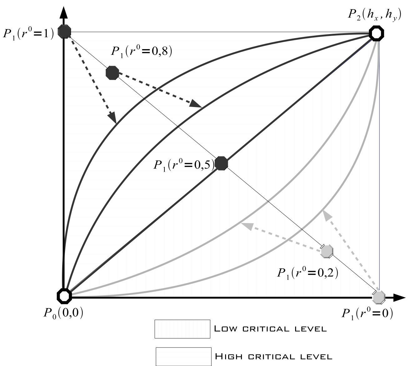
The x axis defines the number of cover sets and the corresponding capture rate can be read on the y axis for a given criticality level (r°). As said previously, the criticality is set to 0.4 in the default omnetpp.ini file. 
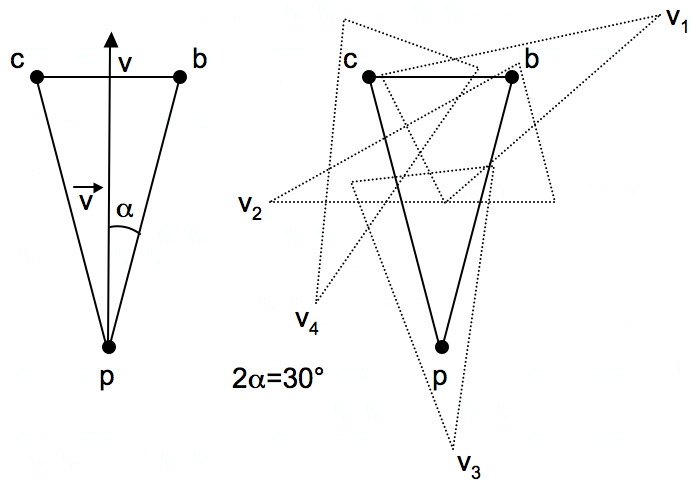
To define the Bezier curves, we need the maximum number of cover sets that will give the maximum frame capture rate (point P2 on the figure). The maximum capture rate in currently set to 6fps in the videoSensorNode.h file. The number of cover set a sensor node can have depends on the node density and on the randomly set line of sight at each simulation run. We set the maximum number of cover sets for a sensor node to 6 as a parameter in the .ned file. Each sensor will read this value at simulation startup. Then the simulation model currently applies a scaling factor of 2 which give 12 as the maximum number of cover sets that will be used to compute the Bezier curves. Therefore, for a maximum number of cover set equal to 12, we can vary r° to have the following capture rates.

#cover    1    2    3    4    5    6    7    8    9    10   11   12
-------------------------------------------------------------------
r0=0.00 0.01 0.05 0.11 0.20 0.33 0.51 0.75 1.07 1.50 2.10 3.04 6.00

r0=0.20 0.14 0.30 0.50 0.73 1.01 1.34 1.73 2.20 2.78 3.52 4.50 6.00
r0=0.40 0.34 0.71 1.09 1.50 1.94 2.41 2.90 3.43 4.00 4.62 5.28 6.00
r0=0.60 0.72 1.38 2.00 2.57 3.10 3.59 4.06 4.50 4.91 5.29 5.66 6.00
r0=0.80 1.50 2.48 3.22 3.80 4.27 4.66 4.99 5.27 5.50 5.70 5.86 6.00
r0=1.00 2.96 3.90 4.50 4.93 5.25 5.49 5.67 5.80 5.89 5.95 5.99 6.00

In the simulation model you could of course change the maximum number of cover set, the maximum capture rate and the getCaptureRate() function in videoSensorNode.cc will determine the correct capture rate depending on the criticality level.

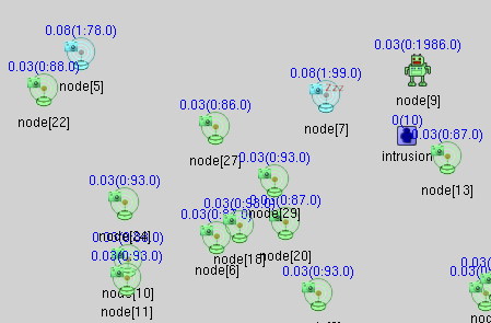
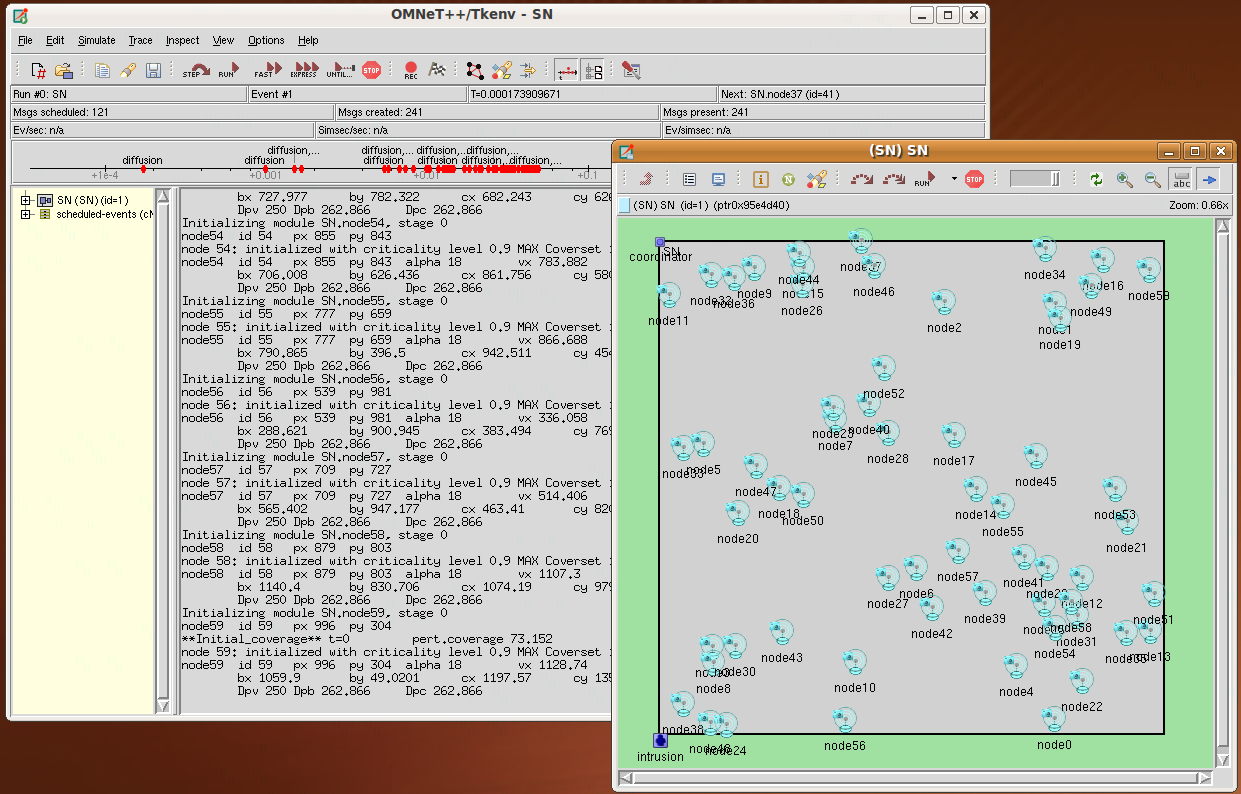
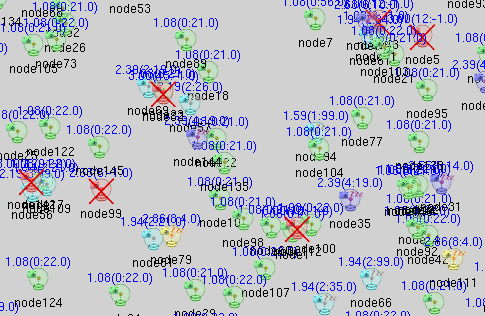
During the simulation the sensor node icon color will change to indicate for each sensor node the number of cover sets that are not dead (not the initial number of found cover sets that is displayed by the information string, see above). The color code is as follows, assuming that N is the maximum number of cover set defined (12 for instance):
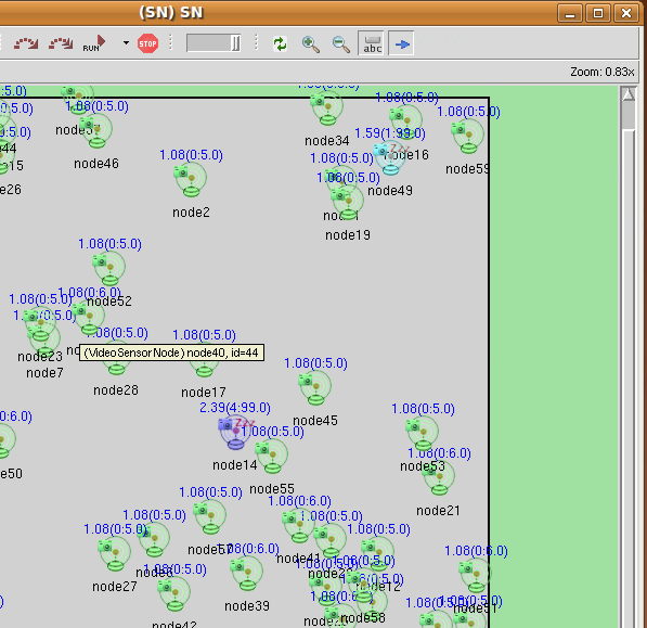
An example is shown below where you can see the green, cyan, blue, yellow and dead icons. The icon color meaning is valid even when the sensor node is inactive. But when the sensor node is dead, there is no more color indication.


Some comments on cover set construction strategies

In order to fully understand the various cover set construction strategies, please refer to [1]. Basically, we define various strategies that takes differents significant points of a sensor v's FoV to determine v's cover set. Various flags defines the behavior of the simulation model.

-DCOVERAGE_WITH_G
uses the triangle points (pbc) and the center of gravity.

-DCOVERAGE_WITH_ALT_G
uses the triangle points (pbc) and 2 alternates points gp and gv

-DCOVERAGE_WITH_ALT_GBC
uses the triangle points (pbc) and 3 alternates points gp, gb and gc

-DCOVERAGE_WITH_XS_AOV
discards point p of the triangle, usually used with the -DCOVERAGE_WITH_ALT_G flag or -DCOVERAGE_WITH_ALT_GBC flag

-DCOVERAGE_MIXED_ANGLEVIEW

defines an heterogeneous scenario where x% of sensor are small AoV sensor and (100-x)% are larger AoV sensor. In the current simulation code, x=80%. Small AoV sensor have an AoV of 20°. Larger AoV sensors have an AoV of 36°.

-DSENSOR_XS_ANGLEVIEW
indicates that all sensors have a small AoV of 20°. Otherwise, all sensors have an AoV of 36° if -DCOVERAGE_MIXED_ANGLEVIEW is not used.

-DCOVERAGE_STATS_ONLY

indicates that the simulation is only interested in determining the cover sets, stops the simulation when the cover set construction phase is finished.

-DCOVERAGE_COMPUTE_PERCOVERSET
as computing the percentage of coverage of each cover set for all sensor is a tie consuming process for the simulation, this flag disables such computation. The cover sets are determined according to the selected cover set construction strategy, but the percentage of coverage is not computed. Then the simulation continues with the scheduling of nodes unless -DCOVERAGE_STATS_ONLY is defined.

Some comments on introducing intrusions in the field

The intrusion module is defined in the ned file. It has an activatedAt parameter that is set by default in the .ned file at t=10s. When intrusions are introduced in the simulation model, the omnetpp.vec file can record the stealth time of each intrusions. The intrusion.cc file defines an intrusion module that defines 2 types of intrusions. The first type is a single point intrusion while the second type is an intrusion rectangle with 8 significant points. There are also 2 types of mobility model. The following flags defines the behavior of the intrusions:

-DWITH_INTRUSION
enables intrusions in the simulation model. Must be defined when using any of the following flags.

-DINTRUSION_SUCC_SCANLINE
define a simple scan line mobility model where an intrusion appears at coordinate (0,10) , moves at a constant velocity of 5m/s (#define INTRUSION_VELOCITY in intrusion.h) toward the right part of the field and reappears at coordinate (0,y+60) when it reaches the right limit. This is performed 10 times as currently coded in the intrusion.cc file. The main statistic provided by this intrusion model is the number of time a sensor sees the intrusion.

-DINTRUSION_RAND_POSITION
defines a simple random intrusion pattern where an intrusion appears at a random position in the field, moves towards the right limit of the field at the velocity of 5m/s (#define INTRUSION_VELOCITY in intrusion.h) unless the field limit is reached in which case a new random position is defined. This process can be repeated a limited number of time but in the intrusion.cc file, this number is set sufficiently high so that once activated intrusions occur until the simulation ends.

-DINTRUSION_STEALTH_TIME
tells the simulation model to compute the stealth time. Usually used with the -DINTRUSION_RAND_POSITION flags. The stealth time is the time during which an intruder can travel in the field without being seen. In the current model, the first intrusion starts at time 10s at a random position in the field. The scan line mobility model is then used with a constant velocity to make the intruder moving to the right part of the field. When the intruder is seen for the first time by a sensor, the stealth time is recorded and the mean stealth time computed. Then a new intrusion appears at another random position. This process is repeated until the simulation ends.

-DINTRUSION_POLYGON
defines an intrusion rectangle instead of a single point intrusion. The rectangle has 8 significant points and is of size 8m by 4m. 4 points are the rectangle's vertices, the other 4 points are the mid-point of the 4 edges. The main statistic provided by this model is to count the number of points of the rectangle that can be seen under various cover set construction stratégies.

If the OMNET++ graphical display is used, the single point intrusion appears with the icon. Its position will also be graphically updated as it moves. An information string will be displayed on top of the icon indicating the number of time the intrusion has been seen, and the number of remaining intrusions.


Some comments on introducing obstacles in the field

Random obstacles can be introduced to investagate occlusions issues. These obstacles are 2D obstacles and are positioned randomly at initialization stage. It is the coordinator that creates the obstacles and if you enable extra graphical support (see below), you will be able to verify that these obstacles actually make some area of the field not covered. For the moment, the number of obstacles is hard coded in the coordNode.cc file but it should be set as a parameter in the .ini file. When there are obstacles, the percentage of coverage may be decrease and an intrusion can be hidden from a camera. The obstacle support is enabled by the -DWITH_OBSTACLES pre-processing flag.

The omnetpp.ini file

As said previously, the omnetpp.ini file is generated by the multipleRun shell script that will be explained below. The default omnetpp.ini file has the following general content:

[General]
network = SN
num-rngs = 1
seed-0-mt = 1799

output-scalar-file = Coverage-60.sca
output-vector-file = omnetpp.vec
 

cmdend-express-mode = yes
cmdenv-status-frequency= 10s

SN.node*.criticalityLevel = 0.9
SN.node*.maxCriticalityLevelPeriod = 5
SN.node*.minCaptureRate = 0.01
SN.field_x = 75
SN.field_y = 75
SN.field_z = 0
SN.numNodes = 60

The interesting part is the section that defines 3 variables used in the simulation model. These parameters belongs to the VideoSensorNode module defined in the Coverage-60.ned file. SN.node*.CriticalityLevel defines the initial criticality level for a sensor node. Then, in the .ned file, each sensor node will use this value to set its criticality level if and only if the -DCRITICALITY_WITH_BEZIER flag is set. Otherwise, the SN.node*.minCaptureRate is used to assign a static and constant capture rate (in frame/s) to all sensor nodes. SN.node*.maxCriticalityLevelPeriod defines a period in second during which a sensor node will stay at the maximum criticality level when dynamic criticality management is used, as explained in the next subsection. SN.field_x and SN.field_y defines the field dimension in meters. SN.numNodes defines the number of nodes. Note that the field's dimension and the number of nodes must match the number of nodes used for generating the .ned file, therefore they can not be changed independently from the .ned file.

Dynamic criticality management

So far, each node is assigned a static criticality level with which a capture rate will be determined according to the number of cover sets as explained previously. 2 preprocessing flags are used to define a more elaborate behavior in which the initial criticality level of sensor nodes is set to a rather low value (0.1 or 0.2) and make it dynamically increase to a maximum value (the SN.node*.criticalityLevel parameter) for a given period of time (the SN.node*.maxCriticalityLevelPeriod parameter) before going back to the initial value. These 2 flags are:

-DDYNAMIC_CRITICALITY_WITH_BEZIER
-DDYNAMIC_REINFORCEMENT_CRITICALITY_WITH_BEZIER

The first flag enables this dynamic behavior. The initial criticality level is defined in the videoSensorNode.h file (#define MIN_CRITICALITY_LEVEL). When an intrusion is detected by a node v, v will run with a criticality level of SN.node*.criticalityLevel for  SN.node*.maxCriticalityLevelPeriod seconds before going back to the initial criticality level. v will also broadcast to its neighbors an alert message. Nodes that receive such an alert message will also set their criticality level to SN.node*.criticalityLevel for  SN.node*.maxCriticalityLevelPeriod seconds before going back to the initial criticality level. No propagation of the alert message is performed yet in the simulation model.

With the second flag, a reinforcement behavior is additionaly introduced:  alerted nodes will not directly set their criticality level to SN.node*.criticalityLevel as described previously. Instead, they first set their criticality level to an intermediate value (#define ALERTED_NODE_CRITICALITY_LEVEL) and will progressively increase this criticality level until they reach SN.node*.criticalityLevel.For the moment, 2 additional alert messages is needed to increase the criticality level by 0.1 (it is hard-coded in the simulation model). For instance, if we assume that ALERTED_NODE_CRITICALITY_LEVEL=0.6 then an alerted nodes will be at the criticality level of 0.8 if it receives 4 more alerted messages (not necessarily from the same node). Nodes that initially detect the intrusion set their criticality level to  SN.node*.criticalityLevel and broadcast an alert message as previously but have to wait a given period of time (#define DYNAMIC_REINFORCEMENT_DEAF_PERIOD) before being able to send new alert messages. This is done mainly to avoid reinforcement for the same intrusion event. In the simulation model, DYNAMIC_REINFORCEMENT_DEAF_PERIOD is set to 2s which with the default velocity of 5m/s usually makes the intrusion moving outside the sensor's FoV.

Generating .ned files

As said previously, ned files for the simulation is generated with the generate utility program found in the nedGeneration folder. It is a simple C++ program that generate, according to a specified number of sensor nodes, the position of the nodes and determine which sensor are connected to which sensor. Additionally, the .ned file also define the structure of the various simulation module: coordinator, intrusion and video sensor node. See the default coverage-60.ned file to get an example.  Generating a .ned file can then be done with:

> nedGeneration/generate 75 > coverage-75.ned
> nedGeneration/generate 75 100 100 > coverage-75-100-100.ned

Be sure to only have one ned file in the whole simulation model directory hierarchy. As OMNET++ can recursively read all .ned files, you may have problems with ned file that (re)define the same network. It is safer to have only one ned file and if you want to keep previous ned files, just rename them with a .save extension.

The program accepts 1 or 3 parameters. The first parameter is the number of nodes. If specified, the next 2 parameters defines the size of the field otherwise the default size of 75m x 75m is used. Connectivity is based on a communication range (set by default in the generate.cpp file to 30m). Then all the connections are set up to generate an appropriate .ned file.

Note that connections between nodes are not drawn in the OMNET++ graphical display because we used the display "o=black,0"; in order to make the OMNET++ display clearer otherwise the graphical view of the entire network is a bit dense.

If you need to add more functionalities in the ned file, such as adding parameters to module, then you may need to modify generate.cpp as well.

Last but not least, we may need to compile generate.cpp in order to get the executable!

> g++ -o generate generate.cpp

Using the multipleRun shell script (may be obsolete with OMNET++ v4)

So far simulation runs are performed manually. It it possible to automatize the procedure, especially when you are varying parameters such as the number of nodes, etc. multipleRun is a Shell script that runs automatically the simulations. Basically, this script generates the omnetpp.ini file that sets up some module parameters , and then runs the simulation executable with several number of nodes. For each number of nodes N, you can set the number of simulation runs you want in order to reduce impacts of randomness. The script will generate a seed.txt file that contains a seed value for the random generator of OMNET++. It is possible to use the same sequence of seeds in order to produce deterministic "random" runs. The current script runs each simulation 3 times. For each number of nodes, the script launches the ned file generator that will produce the coresponding coverage.ned file. Note that the same .ned file is used for all the simulation runs with the same number of nodes. Each run will differ from an other by the seed value.

The script assumes that a Results directory exists. It will then create a Coverage directory where the .sca files will be copied into. Note that for the moment only the .sca file are managed, not the .vec file. When you run N simulations for a given number of nodes, the results of the N runs will be stored in the same .sca file. For example, assuming that you want 3 runs for 75, 100 and 150 nodes, the results of the 3 runs for 75 nodes will be stored in the Coverage-75.sca file. Same thing for the 100 and 150 node scenario. Therefore, in the Coverage folder you will have 3 files: Coverage-75.sca and Coverage-100.sca and Coverage-100.sca . This will make simpler the statistic collection process as will be explained in the next section.

Note that the Coverage folder is erased each time you run multipleRun, so after a whole run has been performed, you need to rename the Coverage folder accordingly. The way I used that script is as follows: (i) produce an executable with the desired behavior with the appropriate pre-processor flags, (ii) run  multipleRun with several node number values, (iii) then rename Coverage folder with a comprehensive name that reflects the behavior of the model. For instance, if the executable uses the COVERAGE_WITH_ALT_G flag with 36° AoV for all sensors, then rename Coverage in Coverage-waG-36.

When multipleRun ends, the coverage.ned, omnetpp.ini and seed.txt files correspond to those of the last run.  You can use them if you want to run the simulation manually. They will be overwritten the next time multipleRun will be run. You can modify multipleRun to your own need. For instance multipleRun could save the coverage.ned associated to the run instead of deleting it, ...

IMPORTANT: usually when you use multipleRun, it is assumed that your simulation model has been debugged and there are no errors. Also, it is appropriate to not use the tkenv of OMNET++ at that stage. Use rather the cmdenv that does not not display the OMNET++ graphical interface that would slow down the runs. To do this, you have to indicate in the Makefile that the cmdenv library should be used instead:

# User interface (uncomment one) (-u option)
USERIF_LIBS=$(CMDENV_LIBS)
#USERIF_LIBS=$(TKENV_LIBS)

Awk scripts, analyzing the results

A very time consuming task is the one of analyzing the results. To help in this task, the awk-script folder contains 3 sample scripts that are used to get gather various statistics from the .sca files. It is assume that you will write your own script that could be based on these sample scripts. The 3 scripts work approximately the same way. In what follows, the extractInfo script is described.

The extractInfo script is a Shell script that uses an awk script called extractInfo.awk. If you look at the shell script, you will see that extractInfo will loop on the node number in the same way multipleRun does. Therefore it is assumed that you use the extractInfo script on the result files written in the Coverage folder (that you should have renamed in a more comprehensive way to avoid that results will be erased at the next call to multipleRun). The entire process of running simulations and building the results is then as follows:

> make clean
> make
> ./multipleRun
> cd Results
> mv Coverage Coverage-waG-36
> cd Coverage-waG-36
> ../../awk-script/extractInfo

The purpose of the script if to get the mean over the 3 runs (or more if you want so) of the recorded values and to make possible the usage of common plotting tools such as gnuplot for instance. So the first step in extractInfo script is to use grep to extract the relevant lines.  For each node number, extractInfo simply extracts from the Coverage-*.sca file the lines that store the statistics for the percentage of coverage for all the cover sets for each simulation runs (recall that all the runs for a given number of nodes are stored in the same .sca file) and the statistics for the number of cover set. These lines contains the "meanPercentageCoversetCoverage" and the "meanNumberCoverset" text strings that will used by grep. For instance, with Coverage-75.sca, extractInfo will produce a Coverage-75.dat that contains only the relevant lines. An example is given below:

scalar "SN.coordinator"     "meanPercentageCoversetCoverage.samples"     5
scalar "SN.coordinator"     "meanPercentageCoversetCoverage.mean"     81.4270666667
scalar "SN.coordinator"     "meanPercentageCoversetCoverage.stddev"     4.96955227919
scalar "SN.coordinator"     "meanPercentageCoversetCoverage.min"     75.1143333333
scalar "SN.coordinator"     "meanPercentageCoversetCoverage.max"     88.041
scalar "SN.coordinator"     "meanNumberCoverset.samples"     5
scalar "SN.coordinator"     "meanNumberCoverset.mean"     2.4
scalar "SN.coordinator"     "meanNumberCoverset.stddev"     2.07364413533
scalar "SN.coordinator"     "meanNumberCoverset.min"     1
scalar "SN.coordinator"     "meanNumberCoverset.max"     6
scalar "SN.coordinator"     "meanPercentageCoversetCoverage.samples"     2
scalar "SN.coordinator"     "meanPercentageCoversetCoverage.mean"     78.3605
scalar "SN.coordinator"     "meanPercentageCoversetCoverage.stddev"     11.3087587515
scalar "SN.coordinator"     "meanPercentageCoversetCoverage.min"     70.364
scalar "SN.coordinator"     "meanPercentageCoversetCoverage.max"     86.357
scalar "SN.coordinator"     "meanNumberCoverset.samples"     2
scalar "SN.coordinator"     "meanNumberCoverset.mean"     2
scalar "SN.coordinator"     "meanNumberCoverset.stddev"     0
scalar "SN.coordinator"     "meanNumberCoverset.min"     2
scalar "SN.coordinator"     "meanNumberCoverset.max"     2
scalar "SN.coordinator"     "meanPercentageCoversetCoverage.samples"     7
scalar "SN.coordinator"     "meanPercentageCoversetCoverage.mean"     86.421047619
scalar "SN.coordinator"     "meanPercentageCoversetCoverage.stddev"     5.70798337509
scalar "SN.coordinator"     "meanPercentageCoversetCoverage.min"     78.888
scalar "SN.coordinator"     "meanPercentageCoversetCoverage.max"     95.568
scalar "SN.coordinator"     "meanNumberCoverset.samples"     7
scalar "SN.coordinator"     "meanNumberCoverset.mean"     2.28571428571
scalar "SN.coordinator"     "meanNumberCoverset.stddev"     1.38013111868
scalar "SN.coordinator"     "meanNumberCoverset.min"     1
scalar "SN.coordinator"     "meanNumberCoverset.max"     4


Then extractInfo uses the extractInfo.awk script which an awk script that will parse the Coverage-75.dat file in order to (i) transform the data which are in a line format to a column format and (ii) make the mean computation, find the max and the min, etc. You could add your own processing either in extractInfo or extractInfo.awk as needed. After extractInfo.awk has been called, there is a file called SynCoverage-75.tmp that will have the following content, assuming that there are 3 runs for each node number scenario.

#nodes & mean%coverage & min,max%coverage & stddev & min,max#coverset & mean#coverset
5 81.4270666667 75.1143333333 88.041 4.96955227919 1 6 2.4
2 78.3605 70.364 86.357 11.3087587515 2 2 2
7 86.421047619 78.888 95.568 5.70798337509 1 4 2.28571428571
nbsample:3 & 6.22 & 82.07 & 74.7888,89.9887 & 6.24 & 1.33333,4 & 2.23

The first line is just a reminder of the meaning of the different column used for the last line. The next 3 lines correspond to the data of the 3 runs in column format. The last line is the results over the 3 runs (nbsample gives the number of runs) where each field corresponds to the meaning indicated by the first line. After extractInfo.awk ends, extractInfo will continue with the next .sca file until all .sca files generated by multipleRun are processed.

Then next step is to collect all the statistics corresponding to all the node number scenario in one file. For instance, if you ran multipleRun with 75, 100, 125, 150 and 175 nodes you will have the following files:

Coverage-75.dat
Coverage-100.dat
Coverage-125.dat
Coverage-150.dat
Coverage-175.dat
SynCoverage-75.tmp
SynCoverage-100.tmp
SynCoverage-125.tmp
SynCoverage-150.tmp
SynCoverage-175.tmp

extractInfo will then use grep once more to get from all the .tmp file the line that begins with "nbsample" to produce a file named according to the current folder name. Assuming that you renamed the Coverage folder in Coverage-waG-36 then you will have a file called SynCoverage-waG-36.dat with the following content:

SynCoverage-100.tmp:nbsample:3 & 11 & 79.22 & 55.4797,96.6882 & 13.16 & 1,5.33333 & 2.05
SynCoverage-125.tmp:nbsample:3 & 18.93 & 79.86 & 49.9902,98.9068 & 12.14 & 1,11.3333 & 3.23
SynCoverage-150.tmp:nbsample:3 & 18.89 & 82.22 & 54.5607,99.0729 & 11.67 & 1,8.66667 & 2.97
SynCoverage-175.tmp:nbsample:3 & 26.67 & 82.07 & 59.2671,99.2611 & 10.17 & 1,22.6667 & 5.32
SynCoverage-75.tmp:nbsample:3 & 6.22 & 82.07 & 74.7888,89.9887 & 6.24 & 1.33333,4 & 2.23
 
Then the last thing that extractInfo will do is to remove the last line in each .tmp file and to rename the .tmp file in a .dat file that you could directly use with gnuplot for instance if you want to plot curves. Note that fields are separated with "&" in the SynCoverage-waG-36.dat file. You can use something else. If you remove the line OFS="&" in the extractInfo.awk script then fields will be separated by a space. The reason "&" is used here is because these statistics were used to fill in Latex tables.

Output .vec file and using plove for plotting curves

OMNET++ v4 does not come with the plove tool anymore. However, I still use this tool that can be found in the OMNET++ v3. In order to use plove with files generated by OMNET++ v4, you need to remove the first few lines The current simulation model records 3 statistic vectors: the percentage of coverage of the initial field, the percentage of active nodes and the stealth time if the required flags for intrusions are defined. These vectors can be plotted with the provided OMNET++ plotting tool plove. Most of the curves in [1,2] have been plotted with plove.

Extra Graphical Support

At the early stage of the model development there was the need of visualizing not only the position of sensor nodes, which is provided by the OMNET++ graphical interface, but also the FoV of each sensor and the initial coverage. This is the purpose of the extra graphical support. If you compile the simulation model with -DDISPLAY_SENSOR then a window will pop-up and will show the sensor nodes spreaded in the field with their respective FoV (left part of the figure below). Then the process of computing the percentage of initial coverage will be shown (right part of the figure below). In the simulation model, 50000 points in the field will be randomly determined and checked whether they are covered by a sensor's FoV or not.


covercover-filled

If you look in the simulation code, you will see that in order to display the sensor nodes some scaling factor must be applied. Also, in order to avoid negative coordinate for the sensor's FoV, which are a bit difficult to handle graphically, there are also a shifting factor applied to the sensor's position. Note that in the current simulation model, this is the shifted value of the sensor's position that is recorded in the .sca file instead of the sensor's position defined in the .ned file. So the whole process is a bit tricky and some constants are defined in display.h. It is however possible to change the depth of view of each sensor (which is by default set to 25m) and the field dimension but be extremely careful.

Technically, the extra graphical support is totally independant from the OMNET++ graphical interface. It uses the SDL library (a nice tutorial can be found here) to set up a graphical environment and to draw points. In coordNode.cc, 2 functions that are used for the graphical display: draw_point() and draw_line(). Then we used a very simple but efficient 2D graphic library written by Carlos Moreno that defines Point, Triangle,... classes for 2D manipulation and drawing. All the drawing uses the draw_point() and draw_line() specific functions that are defined in coordNode.cc. Note that we used the is_inside()feature of this graphic library to know whether a given point is covered by a sensor's FoV which is modeled with a Triangle object.

Note that the Makefile includes extra .o files for the extra graphical support. These .o files are in the geometry folder. It is assumed that these .o files exist and even if you do not use the -DDISPLAY_SENSOR flag, these .o files are needed in the Makefile! They can be obtained by running make obj in the geometry folder. In this folder you will also find some test program written for debugging purpose. One is called viewFOV and accepts 2 parameters: the number of nodes and the depth of view. viewFOV will then display randomly placed sensors with their respective FoV. It is a very simple program that shows the capabilities of the SDL library and the 2D graphic library. You can run viewFOV with:

> ./viewFOV 125 75

where 125 is the number of sensor nodes and 75 means 25m for the depth of view.

When obstacles are introduced with the -DWITH_OBSTACLES pre-processing flag, obstacles will be shown in red and then the simulation will wait (in the terminal window) for key press to continue with the sensor's FoV visualization and initial coverage computation (in green).

obstaclesobstacles-filled

Debugging

I use the insight GUI front-end to gdb for debugging purposes. By default, OMNET++ comes with a configure.user file that has the following lines:

#CFLAGS='-g -Wno-unused'
#CFLAGS='-g -Wall'
#CFLAGS='-gstabs+3 -Wall'
CFLAGS='-O2 -DNDEBUG=1'

To enable advanced debugging feature, just use CFLAGS='-gstabs+3 -Wall' and rebuild OMNET++, otherwise only your source code will be available. An additional tools for checking memory leaks that I used is valgrind. The current simulation model under OMNET++ has been tested with valgrind and so far, no memory leaks have been reported.

Using the Castalia framework

The simulation model can be used with the Castalia framework in order to benefit from the advanced radio communication channel modeling. The major differences for the user are the structure of the ned file and the content of the omnetpp.ini file. For the developper, the main difference is how packets are sent: without Castalia, packets were sent using direct communication channels to other sensor nodes, with Castalia, all packets are sent to the communication module which in turn uses the wireless channel provided by the Castalia fremawork. Actually, it is expected that the Castalia framework will become the main simulation model. However, as the same code source is used, all the cover set construction steps and criticality management (static and dynamic) remain the same. Compiling for Castalia needs the -DCASTALIA flag. This specific page will describe in more details the general structure of the simulation model with Castalia.

Future works

Many parameters could be put in the .ned file (generated by the generate program) or in the omnetpp.ini (probably better) file generated by the multipleRun script. With Castalia, some of the parameters have already been integrated to the omnetpp.ini file but it is possible to go further.

References

[1] C. Pham and A. Makhoul. "Performance study of multiple cover-set strategies for mission-critical video surveillance with wireless video sensors". Proceedings of the IEEE WiMob 2010.

[2] C. Pham. "Fast event detection in mission-critical surveillance with wireless video sensor networks". Proceedings of the IEEE RIVF 2010.

[3] A. Makhoul, R. Saadi and C. Pham. "Risk Management in Intrusion Detection Applications with Wireless Video Sensor Networks". Proceedings of the IEEE WCNC international conference, Sydney, Australia, April 2010.

Acknowledgements

The very first version of the video sensor simulation model has been written by A. Makhoul when he was a postdoc fellow at the University of Pau, sep.2008-aug.2009.